
Physical intuition of Floquet periodicity
Published:
When analyzing wave propagation inside a periodic structure, one may consider the analysis over a single section or a unit cell, instead of the complete domain, by considering the appropriate periodicity at the boundaries. This approach reduces the domain of analysis and simplifies the problem.
Bloch theorem describes the behavior of the wave propagation inside a periodic structure are analogous to plane wave modulated by a periodic function, which can be described mathematically as
\[\psi(\mathbf{r})=\mathrm{e}^{\mathrm{ik} \cdot \mathbf{r}} u(\mathbf{r})\]where, \(\psi(\mathbf{r})\) is the overall field {combination of plane wave and periodic function}
\(\mathrm{e}^{\mathrm{ik} \cdot \mathbf{r}}\) is the plane wave {Bloch wave vector}
\(u(\mathbf{r})\) is the envelop function {takes the periodicity and symmetry of the periodic structure}.
Bloch-floquet theory or periodicity provides a methodology to analyze the wave propagation by just considering a single unit cell and applying the following boundary condition as
\[u(\mathbf{r}+\mathbf{R})=u(\mathbf{r}) e^{i \mathbf{k} \mathbf{r}}\]where, \(u()\) is the field variable, \(\mathbf{r}\) is the spatial coordinates of the boundaries, \(R\) is the periodicity, and \(k\) is the wavenumber.
Wavenumber can be defined as the number of waves per unit length and is written as
\[k = \frac{1}{\lambda}\]A structure is considered periodic if its material properties repeat after certain intervals. For example in case of permittivity \varepsilon $(\mathbf{r})$ can be defined as
\[\varepsilon( \mathbf{r} + \mathbf{t_{pqr}} ) = \varepsilon (\mathbf{r})\]where, \(\mathbf {t_{pqr}}\) is the periodicity of the structure and \(\varepsilon\) is the permittivity of the material.
Consider a unit cell as shown in below having periodicity \(R\) equal to 1 and the boundary value at left and right be \(u_l\) and \(u_r\), respectively. Then above equation reduces to
\[u(\mathbf{r}+1)=u(\mathbf{r}) e^{i \mathbf{k} \mathbf{r}}\]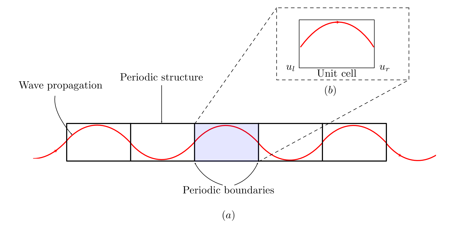
Considering the value of \(r\) to be 1 at the left most side, then above equation becomes
\[u_r=u_l e^{i \mathbf{k}}\]which can also be written as,
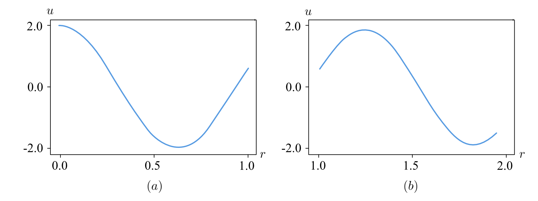
\[u_r = u_l [cos(k) + i* sin(k)]\]The value \(u_l[cos(k)]\) of the real part of field variable \(u(r)\) is plotted for two consecutive unit cells for a wave having wave number \(k\) equals to 0.8. From the plots shown below, it can be seen that the field variables takes the periodicity of wave \(cos(k)\) and the generates the value based on initial boundary condition \(u_l\).
References -